In the CHOMP[1] paper, the obstacle cost is defined in Eq. 23 of the paper:
\[\tag{1} \mathcal{F}_\text{obs} [\xi] = \int_0^1 \int_{u \in \mathcal{B}} c(x(\xi(t), u)) \left\lVert\frac{d}{dt} x(\xi(t), u)\right\rVert \,du \,dt\]The functional gradient is given in Eq. 24 as:
\[\tag{2} \bar \nabla \mathcal{F}_\text{obs} [\xi] = \frac{\partial v}{\partial \xi} - \frac{d}{dt}\frac{\partial v}{\partial \xi'}\]where \(v\) is the everything inside the time integral of Eq. 23 of the paper, i.e.,
\[\tag{3} v = \int_{u \in \mathcal{B}} c(x(\xi(t), u)) \left\lVert\frac{d}{dt} x(\xi(t), u)\right\rVert \,du\]The paper gives the functional gradient of Eq. 1 in Eq. 25 as:
\[\tag{4} \bar \nabla \mathcal{F}_\text{obs} [\xi] = \int_{u \in \mathcal{B}}J^\top\left( \left\lVert x'\right\rVert \left( \left(I - \hat{x'}\hat{x'}^\top\right) \nabla c - c\kappa \right)\right) \,du\]where
\[\kappa = \frac{1}{\left\lVert x'\right\rVert^2} \left(I - \hat{x'}\hat{x'}^\top\right)x''\]We will derive \(\bar \nabla \mathcal{F}_\text{obs} [\xi]\).
Preliminaries
Notation
-
\(x(q, u) : \mathbb{R}^w \rightarrow \mathcal{B}\) is the forward kinematic function of the robot, given a point on the body \(u \in \mathcal{B}\) and its configuration \(q\).
-
\(\xi \approx (q_1^\top, q_2^\top, ..., q_n^\top)^\top\) is the trajectory, which is basically a matrix of the joint angles.
-
\((\cdot)'\) is the first derivative with respect to a line integral. In this case, the line integral is defined with respect to time \(t\), therefore it can also be seen as \(\frac{d (\cdot)}{d t}\), i.e., the velocity, and \((\cdot)''\) the acceleration, etc.
-
\(\hat{x} = \frac{x}{\left\lVert x\right\rVert}\) is the normalized vector of x.
-
\(J = \frac{\partial x}{\partial \xi}\) is the kinematic Jacobian that relates changes in state to joint angles.
-
Partial gradient notation: \(\nabla c = \frac{\partial c}{\partial x}\)
Simplifying equations
We will use these simplfying equations in the derivation.
\[\tag{5} \frac{\partial \left\lVert x(z)\right\rVert}{\partial z} = \frac{\partial}{\partial z}(x^\top x)^{\frac{1}{2}} = \frac{1}{2}(x^\top x)^{-\frac{1}{2}} \frac{\partial (x^\top x)}{\partial z} = \frac{1}{2}\frac{1}{(x^\top x)^{\frac{1}{2}}} 2x^\top\frac{\partial x}{\partial z} = \frac{1}{\left\lVert x\right\rVert} x^\top\frac{\partial x}{\partial z} = \hat x^\top\frac{\partial x}{\partial z}\] \[\tag{6} \frac{\partial}{\partial t}{\hat x} = \frac{\partial}{\partial t} \frac{x}{\left\lVert x\right\rVert} = \frac{x'}{\left\lVert x\right\rVert} - \frac{x x^\top x'}{\left\lVert x\right\rVert^3} = \frac{x'}{\left\lVert x\right\rVert} - \frac{x}{\left\lVert x\right\rVert}\frac{x^\top}{\left\lVert x\right\rVert}\frac{x'}{\left\lVert x\right\rVert} = \frac{x'}{\left\lVert x\right\rVert} - \hat x \hat x^\top\frac{x'}{\left\lVert x\right\rVert} = (I - \hat x \hat x^\top) \frac{x'}{\left\lVert x\right\rVert}\]Derivation
Dropping dependencies of \(c\), \(x\) on \(\xi, u\), we have
\[v = \int_{u \in \mathcal{B}} \left( c \left\lVert x'\right\rVert \right) \,du\]Then
\[\begin{aligned} \bar \nabla \mathcal{F}_\text{obs} [\xi] &= \frac{\partial v}{\partial \xi} - \frac{d}{dt}\frac{\partial v}{\partial \xi'}\\ &=\frac{\partial}{\partial \xi} \int_{u \in \mathcal{B}} \left( c \left\lVert x'\right\rVert \right) \,du - \frac{d}{dt}\frac{\partial}{\partial \xi'} \int_{u \in \mathcal{B}} \left( c \left\lVert x'\right\rVert \right)\,du \\ &= \int_{u \in \mathcal{B}} \left( \frac{\partial}{\partial \xi} \left( c \left\lVert x'\right\rVert \right) - \frac{d}{dt}\frac{\partial}{\partial \xi'} \left( c \left\lVert x'\right\rVert \right) \right) \,du && \text{\footnotesize exchange the integral and derivatives}\end{aligned}\]We can compute the above integral in parts:
\[\tag{7} \begin{aligned} \bar \nabla \mathcal{F}_\text{obs} [\xi] &= \int_{u \in \mathcal{B}} \biggl( \underbrace{ \frac{\partial}{\partial \xi} c \left\lVert x'\right\rVert}_{\text{Part 1}} - \underbrace{\frac{d}{dt}\frac{\partial}{\partial \xi'} c \left\lVert x'\right\rVert }_{\text{Part 2}} \biggr) \,du\end{aligned}\]Now we will compute Part 1 and Part 2 separately.
Part 1
Using the chain rule,
\[\begin{aligned} \frac{\partial}{\partial \xi} \left(c \left\lVert x'\right\rVert \right) &= \underbrace{\frac{\partial c}{\partial x}}_{\mathclap{\nabla c}} \underbrace{\frac{\partial x}{\partial \xi}}_{\mathclap{J}} \left\lVert x'\right\rVert + c \underbrace{\frac{\partial \left\lVert x'\right\rVert}{\partial \xi}}_{\hat{x'}^\top\, \frac{\partial x'}{\partial \xi} \mathrlap{\text{\footnotesize using Eq. 5}}} \\ &= \nabla c J \left\lVert x'\right\rVert + c\,\hat{x'}^\top\, \frac{\partial x'}{\partial \xi} \tag{8}\end{aligned}\]Part 2
\[\begin{aligned} \frac{d}{dt}\frac{\partial}{\partial \xi'} c \left\lVert x'\right\rVert &= \frac{d}{dt}\biggl( \underbrace{\frac{\partial c}{\partial x}}_{\mathclap{\nabla c}} \frac{\partial x}{\partial \xi'} \left\lVert x'\right\rVert + c \frac{\partial \left\lVert x'\right\rVert}{\partial \xi'}\biggr)\\ \frac{d}{dt}\frac{\partial}{\partial \xi'} c \left\lVert x'\right\rVert &= \frac{d}{dt}\biggl( \nabla c \frac{\partial x}{\partial \xi'} \left\lVert x'\right\rVert + c \underbrace{\frac{\partial \left\lVert x'\right\rVert}{\partial \xi'}}\biggr) \tag{8}\end{aligned}\]Let us deal with the rightmost term first:
\[\begin{aligned} \frac{\partial \left\lVert x'\right\rVert}{\partial \xi'} &=\frac{x'^\top}{\left\lVert x'\right\rVert} \cdot \frac{\partial}{\partial \xi'}(x') && \text{\footnotesize using Eq.5}\\ &=\frac{x'^\top}{\left\lVert x'\right\rVert} \cdot \frac{\partial}{\partial \xi'}\biggl(\frac{d x}{d t}\biggr)\\ &=\frac{x'^\top}{\left\lVert x'\right\rVert} \cdot \frac{\partial}{\partial \xi'}\biggl(\frac{\partial x}{\partial \xi} \frac{\partial \xi}{\partial t}\biggr)\\ &=\frac{x'^\top}{\left\lVert x'\right\rVert} \cdot \underbrace{\frac{\partial}{\partial \xi'}\biggl(\frac{\partial x}{\partial \xi} \xi'} \biggr) && \text{\footnotesize Now if we take the derivative of this second term, we have}\\ &=\frac{x'^\top}{\left\lVert x'\right\rVert} \cdot \frac{\partial x}{\partial \xi} \\ & = \hat{x'}^\top J\end{aligned}\]Substituting back in Eq. 8, we have
\[\begin{aligned} \frac{d}{dt}\frac{\partial}{\partial \xi'} c \left\lVert x'\right\rVert &= \frac{d}{dt}\biggl( \nabla c \frac{\partial x}{\partial \xi'} \left\lVert x'\right\rVert + c \, \hat{x'}^\top J \biggr)\end{aligned}\]Applying the chain rule to the derivative with respect to time, we have:
\[\begin{aligned} \frac{d}{dt}\frac{\partial}{\partial \xi'} c \left\lVert x'\right\rVert &= \underbrace{\frac{d}{dt}\biggl( \nabla c \frac{\partial x}{\partial \xi'} \left\lVert x'\right\rVert\biggr)}_{\textbf{A}} + \underbrace{\frac{d}{dt}\biggl( c \, \hat{x'}^\top J \biggr)}_{\textbf{B}}\end{aligned}\]We deal with and separately. Applying the chain rule to :
\[\begin{aligned} \textbf{A} \quad \frac{d}{dt}\biggl( \nabla c \frac{\partial x}{\partial \xi'} \left\lVert x'\right\rVert\biggr) & = \frac{d (\nabla c)}{d t} \frac{\partial x}{\partial \xi'} \left\lVert x'\right\rVert + \nabla c \frac{d}{dt}\biggl(\frac{\partial x}{\partial \xi'}\biggr)\left\lVert x'\right\rVert + \nabla c \frac{\partial x}{\partial \xi'} \frac{d \left\lVert x'\right\rVert}{d t}\\ & = \frac{d (\nabla c)}{d t} \frac{\partial x}{\partial \xi'} \left\lVert x'\right\rVert + \nabla c \frac{d}{dt}\biggl(\frac{\partial x}{\partial \xi'}\biggr)\left\lVert x'\right\rVert + \nabla c \frac{\partial x}{\partial \xi'} \underbrace{\frac{d \left\lVert x'\right\rVert}{d t}}\\ & = \frac{d (\nabla c)}{d t} \frac{\partial x}{\partial \xi'} \left\lVert x'\right\rVert + \nabla c \frac{d}{dt}\biggl(\frac{\partial x}{\partial \xi'}\biggr)\left\lVert x'\right\rVert + \nabla c \frac{\partial x}{\partial \xi'} \underbrace{\hat{x'}^\top\frac{\partial x'}{\partial t}}\\ & = \frac{d (\nabla c)}{d t} \frac{\partial x}{\partial \xi'} \left\lVert x'\right\rVert + \nabla c \frac{d}{dt}\biggl(\frac{\partial x}{\partial \xi'}\biggr)\left\lVert x'\right\rVert + \nabla c \frac{\partial x}{\partial \xi'} \biggl(\hat{x'}^\top x'' \biggr)\end{aligned}\]Now, we apply the chain rule to :
\[\begin{aligned} \textbf{B} \qquad \frac{d}{dt}\biggl( c \, \hat{x'}^\top J \biggr) &= \frac{d c}{d t} \, \hat{x'}^\top J + c \, \frac{d}{dt}\biggl( \hat{x'}^\top\biggr) J + c \, \hat{x'}^\top\frac{d J}{d t}\\ &= \underbrace{\frac{d c}{d t}} \, \hat{x'}^\top J + c \, \underbrace{\frac{d}{dt}\biggl( \hat{x'}^\top\biggr)} J + c \, \hat{x'}^\top\frac{d J}{d t}\\ &= \underbrace{\frac{\partial c}{\partial x}\frac{\partial x}{\partial t}} \, \hat{x'}^\top J + c \, \underbrace{(I - \hat{x'}\hat{x'}^\top) \frac{x''}{\left\lVert x'\right\rVert}}_{\text{\footnotesize using Eq.6}} J + c \, \hat{x'}^\top\frac{d J}{d t}\\ &= \nabla c \, x' \, \hat{x'}^\top J + c \, (I - \hat{x'}\hat{x'}^\top) \frac{x''}{\left\lVert x'\right\rVert} J + c \, \hat{x'}^\top\frac{d J}{d t}\end{aligned}\]Putting \(\textbf{A}\) and \(\textbf{B}\) together:
\[\begin{aligned} \frac{d}{dt}\frac{\partial}{\partial \xi'} c \left\lVert x'\right\rVert &= \textbf{A} + \textbf{B}\\ &= \biggl( \frac{d (\nabla c)}{d t} \frac{\partial x}{\partial \xi'} \left\lVert x'\right\rVert + \nabla c \frac{d}{dt}\biggl(\frac{\partial x}{\partial \xi'}\biggr)\left\lVert x'\right\rVert + \nabla c \frac{\partial x}{\partial \xi'} \biggl(\hat{x'}^\top x'' \biggr)\biggr)\\ & + \biggl( \nabla c \, x' \, \hat{x'}^\top J + c \, (I - \hat{x'}\hat{x'}^\top) \frac{x''}{\left\lVert x'\right\rVert} J + c \, \hat{x'}^\top\frac{d J}{d t} \biggr) \tag{9}\end{aligned}\]Together
Now, let us put Part 1 (Eq. 8) and Part 2 (Eq. 9) together:
\[\begin{aligned} \biggl( \underbrace{ \frac{\partial}{\partial \xi} c \left\lVert x'\right\rVert}_{\text{Part 1}}& - \underbrace{\frac{d}{dt}\frac{\partial}{\partial \xi'} c \left\lVert x'\right\rVert }_{\text{Part 2}} \biggr) \\ &= \underbrace{\nabla c \, J \left\lVert x'\right\rVert + c\,\hat{x'}^\top\, \frac{\partial x'}{\partial \xi}}_{\text{Part 1}} -\biggl( \underbrace{ \frac{d (\nabla c)}{d t} \frac{\partial x}{\partial \xi'} \left\lVert x'\right\rVert + \nabla c \frac{d}{dt}\biggl(\frac{\partial x}{\partial \xi'}\biggr)\left\lVert x'\right\rVert + \nabla c \frac{\partial x}{\partial \xi'} \biggl(\hat{x'}^\top x'' \biggr)}_{\textbf{A}}\\ & + \underbrace{\nabla c \, x' \, \hat{x'}^\top J + c \, (I - \hat{x'}\hat{x'}^\top) \frac{x''}{\left\lVert x'\right\rVert} J + c \, \hat{x'}^\top\frac{d J}{d t}}_{\textbf{B}} \biggr)\end{aligned}\]If we assume \(\frac{\partial x'}{\partial \xi} = 0\), \(\frac{\partial x}{\partial \xi'} = 0\), \(\frac{d}{dt}J = 0\), (and consequently \(\frac{d}{dt}\frac{\partial x}{\partial \xi'} = 0\)), then we can greatly simplify this expression:
\[\begin{aligned} & \nabla c J \left\lVert x'\right\rVert + \cancel{c\,\hat{x'}^\top\, \frac{\partial x'}{\partial \xi}} - \cancel{\frac{d (\nabla c)}{d t} \frac{\partial x}{\partial \xi'} \left\lVert x'\right\rVert} - \cancel{\nabla c \frac{d}{dt}\biggl(\frac{\partial x}{\partial \xi'}\biggr)\left\lVert x'\right\rVert} - \cancel{\nabla c \frac{\partial x}{\partial \xi'} \biggl(\hat{x'}^\top x'' \biggr)} \\ & - \nabla c \, x' \, \hat{x'}^\top J - c \, (I - \hat{x'}\hat{x'}^\top) \frac{x''}{\left\lVert x'\right\rVert} J - \cancel{c \, \hat{x'}^\top\frac{d J}{d t}}\\ &\qquad \qquad \qquad = \nabla c J \left\lVert x'\right\rVert - \nabla c \, x' \, \hat{x'}^\top J - c \, (I - \hat{x'}\hat{x'}^\top) \frac{x''}{\left\lVert x'\right\rVert} J \tag{10}\end{aligned}\]Now, we rearrange the last equation (Eq. 10):
\[\begin{aligned} \nabla c J \left\lVert x'\right\rVert - \nabla c \, &x' \, \hat{x'}^\top J - c \, (I - \hat{x'}\hat{x'}^\top) \frac{x''}{\left\lVert x'\right\rVert} J\\ &= J^\top\biggl( \biggl(\left\lVert x'\right\rVert - x' \, \hat{x'}^\top\biggr)\nabla c - c (I - \hat{x'}\hat{x'}^\top) \frac{x''}{\left\lVert x'\right\rVert}\biggr)\\ &= J^\top\biggl( \biggl(\left\lVert x'\right\rVert - x' \, \hat{x'}^\top\underbrace{\frac{\left\lVert x'\right\rVert}{\left\lVert x'\right\rVert}}_{\mathclap{\text{\footnotesize multiply the numerator and denominator by the same thing}}} \biggr)\nabla c - c (I - \hat{x'}\hat{x'}^\top) \frac{x''}{\left\lVert x'\right\rVert}\biggr)\\ &= J^\top\biggl( \biggl(\left\lVert x'\right\rVert - \left\lVert x'\right\rVert\frac{x'}{\left\lVert x'\right\rVert} \, \hat{x'}^\top\biggr)\nabla c - c (I - \hat{x'}\hat{x'}^\top) \frac{x''}{\left\lVert x'\right\rVert}\biggr)\\ &= J^\top\biggl( \biggl(\left\lVert x'\right\rVert - \left\lVert x'\right\rVert \hat{x'} \hat{x'}^\top\biggr)\nabla c - c (I - \hat{x'}\hat{x'}^\top) \frac{x''}{\left\lVert x'\right\rVert}\biggr)\\ &= J^\top\biggl( \left\lVert x'\right\rVert(I - \hat{x'} \hat{x'}^\top)\nabla c - c (I - \hat{x'}\hat{x'}^\top) \frac{x''}{\left\lVert x'\right\rVert}\underbrace{\frac{\left\lVert x'\right\rVert}{\left\lVert x'\right\rVert}}_{\mathclap{\text{\footnotesize same trick}}}\biggr)\\ &= J^\top\biggl( \left\lVert x'\right\rVert(I - \hat{x'} \hat{x'}^\top)\nabla c - c (I - \hat{x'}\hat{x'}^\top) \frac{x''}{\left\lVert x'\right\rVert^2}\left\lVert x'\right\rVert\biggr)\\ &= J^\top\biggl( \left\lVert x'\right\rVert\biggl((I - \hat{x'} \hat{x'}^\top)\nabla c - c \underbrace{(I - \hat{x'}\hat{x'}^\top) \frac{x''}{\left\lVert x'\right\rVert^2}}_{\kappa} \biggr) \biggr)\\ \text{this gives us:} & \\ \biggl( \frac{\partial}{\partial \xi} c \left\lVert x'\right\rVert -\frac{d}{dt}\frac{\partial}{\partial \xi'} c \left\lVert x'\right\rVert\biggr) & = J^\top\biggl( \left\lVert x'\right\rVert\biggl((I - \hat{x'} \hat{x'}^\top)\nabla c - c \kappa \biggr) \biggr) \tag{11}\end{aligned}\]Now put Eq. 10 into Eq. 7} to get the final form:
\[\begin{aligned} \bar \nabla \mathcal{F}_\text{obs} [\xi] &= \int_{u \in \mathcal{B}} \biggl( \frac{\partial}{\partial \xi} c \left\lVert x'\right\rVert -\frac{d}{dt}\frac{\partial}{\partial \xi'} c \left\lVert x'\right\rVert \biggr) \,du\\ &= \int_{u \in \mathcal{B}}J^\top\biggl( \left\lVert x'\right\rVert\biggl((I - \hat{x'} \hat{x'}^\top)\nabla c - c \kappa \biggr) \biggr) \,du\end{aligned}\]where
\[\kappa = \frac{1}{\left\lVert x'\right\rVert^2} \left(I - \hat{x'}\hat{x'}^\top\right)x''\]Compare this solution with Eq.4, which is Eq. 25 in the paper.
Notes
The form of Eq. 1 is similar to a form of the Elastic Band model which was first introduced by Sean Quinlan. Quinlan’s thesis introduces a elastic bands using a constant elastic tension force, which is used to model deforming a collision-free path. In Section 3.7 of his thesis, a simplified objective function is introduced as
\[v_{int} = k \left\lVert\mathbf{c}'\right\rVert\]which is the internal density function. The corresponding contraction force,
\[\tag{12} \mathbf{f}_{int}(s) = - \bar \nabla v_{int} = \frac{d }{d s} \frac{\partial v_{int}}{\partial \mathbf{c}'}\]is similar to the gradient equation (Eq. 2). Note that the spring constant \(k\) in \(v_{int}\) is constant, whereas the \(v\) in the CHOMP formulation (Eq. 3) the cost \(c\) is dependent on the state \(x\). The solution to Eq.12 is:
\[\mathbf{f}_{int}(s) = \frac{k}{\left\lVert\mathbf{c}'\right\rVert^2} \biggl( \mathbf{c}'' - \frac{\mathbf{c}'' \cdot \mathbf{c}'}{\left\lVert\mathbf{c}'\right\rVert^2}\mathbf{c}'\biggr)\]For the exact derivation, please see Section 3 of Quinlan’s thesis[2].
References
-
M. Zucker, N. Ratliff, A. D. Dragan, M. Pivtoraiko, M. Klingensmith, C. M. Dellin, J. A. Bagnell, and S. S. Srinivasa, “Chomp: Covariant hamiltonian optimization for motion planning,” The International Journal of Robotics Research, vol. 32, no. 9-10, pp. 1164–1193, 2013.
-
S. Quinlan, Real-time modification of collision-free paths. Page 5 of 5 Stanford University, 1994, no. 1537
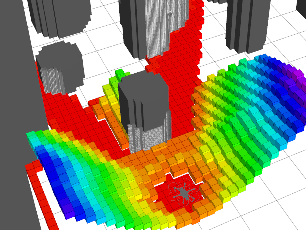
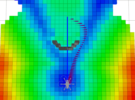
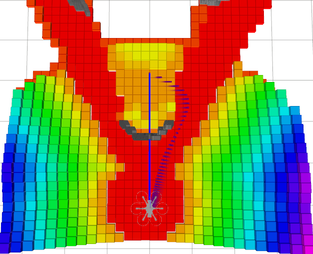
Note about the figures: Notice that a forward sensor scan does not capture the interior of an obstacle. This is a problem for another blog post…